The Four Realms of Neural Networks

In xianxia novels, a cultivator climbs through realms. Each step up reveals a deeper layer of reality that was always present — just invisible from below. Neural networks work the same way. Below is a four-realm reading of what deep learning actually is. Each realm is a useful lens, and each one brings out structure the lower realm cannot express. By the time we reach the top, one specific shape of AGI becomes very hard to avoid.

金刚境 — The Diamond Realm: A neural network is a PDE solver

Take the simplest possible neural-network claim seriously. Forward propagation is iterated integration; backpropagation is residual correction; activation functions inject high-order nonlinearity. Sum it up and you are looking at a numerical solver for a high-order nonlinear partial differential equation.

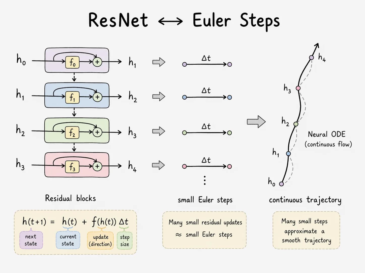
This is not metaphor. A Transformer block — attention plus MLP, each with a residual connection —

is Euler's method for an ordinary differential equation. Chen et al. (2018) made this rigorous for residual networks in Neural Ordinary Differential Equations: replace a discrete residual stack with a continuous adaptive ODE solver and you get a working neural network with constant memory cost. The same residual shape sits inside every Transformer block. Depth becomes integration time.

Backpropagation, for its part, is not a machine-learning invention. It is the adjoint sensitivity method — a 1960s control-theory technique for propagating gradients backward through a dynamical system. Linnainmaa wrote it down in 1970. Werbos applied it to neural nets in 1974. But it was the 1986 Nature paper by Rumelhart, Hinton — my professor at the University of Toronto, and a 2018 Turing Award laureate — and Williams, Learning representations by back-propagating errors, that showed the trick scaled and mattered. Every gradient update in every model shipping today is a direct descendant of those three pages.

Activation functions earn their own sentence. Without them, any stack of linear layers collapses to a single affine map — Cybenko's 1989 universal approximation theorem requires nonlinearity. The sigmoid, tanh, ReLU, GELU you see in code are not aesthetic choices; they are the nonlinear perturbation that prevents a 200-layer network from being algebraically equivalent to a 1-layer one.

This reading is structural — no one has written down the PDE a given Transformer is solving, and there may not be one in closed form. What the view does give you is a one-to-one correspondence of parts: iterated forward steps, adjoint-method gradients, nonlinear coefficients, boundary conditions. Stated cleanly: a Transformer behaves like a PDE whose coefficients are learned by gradient descent, and whose boundary conditions are your prompt.

This is a useful thing to see. It is also the lowest realm, because it tells you what the machine is computing without telling you why the computation works.

指玄境 — The Pointing-Mystery Realm: Training is geometric flattening of a manifold

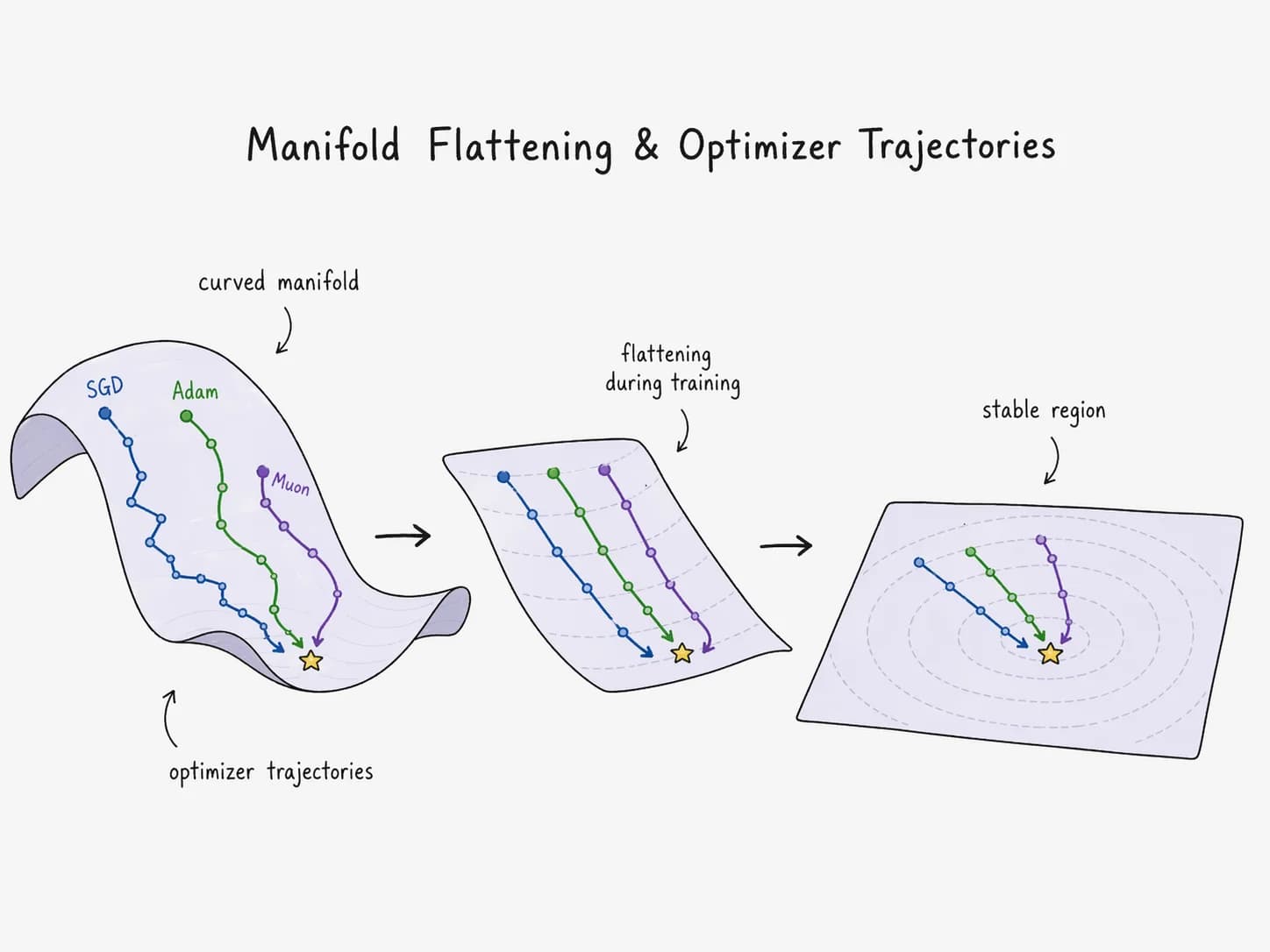
Fold a sheet of paper into an airplane. Now fold ten sheets each into different airplanes, stack them in the air, and ask: how would you flatten all of them into a single 2D plane such that the original creases still let you tell each airplane apart?

This is what training a neural network does. Each class of input — cats, dogs, the word France — lives on a curved, locally Euclidean submanifold inside the ambient input space. Raw pixels or tokens tangle these manifolds together. Training progressively unfolds them until they are linearly separable.

Christopher Olah's Neural Networks, Manifolds, and Topology (2014) is still the cleanest visualization of this picture. The machinery factors into three elementary moves:

• Linear transform → flatten and rotate. An affine layer $Wx + b$ reorients the ambient space — rotation, scaling, shear, projection, translation are all on the table.
• Activation → bend. A nonlinearity locally stretches or compresses along each coordinate, putting curvature where there was none.
• MLP dimension shift → cut and re-glue. Changing the hidden dimension is topologically analogous to embedding the manifold in a higher-dimensional ambient space where tangled submanifolds can be pulled apart.

A trained weight matrix, under this reading, is a choreography: where to transform, how hard to bend, and where to translate. The loss landscape has not one optimum but many — N > 1 fixed points that all flatten the manifolds acceptably well. Training is the geometric search for any one of them.

Gen-Hua Shi's Deep Manifold framework makes this mathematically explicit: neural networks are "learnable numerical computation" over stacks of piecewise-smooth manifolds, grounded in fixed-point theory. The framework's claim — that a neural network is the first computational object whose structure is defined by counting fixed points over nested manifolds — lines up exactly with the geometric picture above. It is the formal statement of what Olah showed visually.

The strongest recent signal that geometry is the right prior comes from optimizers. Muon, introduced by Keller Jordan in late 2024, post-processes each SGD momentum update by running a Newton–Schulz iteration that approximately replaces the update matrix with its nearest semi-orthogonal counterpart — effectively projecting the update onto $UV^T$ from the SVD. Orthogonal updates are isometric: they rotate the weight-space tangent vector without rescaling any direction. SGD is axis-aligned. Adam is per-coordinate rescaling that does not preserve the geometric structure the manifold view cares about. Muon treats the weight matrix as what it actually is — a geometric object — and updates it accordingly. On NanoGPT speedruns it wins. The lesson generalizes: the right inductive bias for a 2D weight matrix is a geometric one.

天象境 — The Heavenly-Phenomenon Realm: Weights are a connection on a fiber bundle over the data manifold

The geometric picture is still too flat. Real data is not just a manifold in input space — it is a manifold with structure attached at every point. To see that structure, we need the language of gauge theory and fiber bundles.

Start with a name. Chen Shing-Shen (陈省身, 1911–2004) was a Chinese-American geometer whose work on characteristic classes — the Chern classes, the Chern–Simons form, the Chern–Gauss–Bonnet theorem — underpins essentially all of modern gauge theory and much of string theory. He was Yau Shing-Tung's doctoral advisor. His fiber-bundle machinery is what physicists use to describe every fundamental force we know.

In physics:

• Electromagnetism is a U(1) gauge theory; the gauge field is the electromagnetic potential.
• Weak force is SU(2). Strong force is SU(3). The Standard Model is SU(3) × SU(2) × U(1).
• Gravity curves spacetime — a connection on the tangent bundle of the 4-manifold we live on.

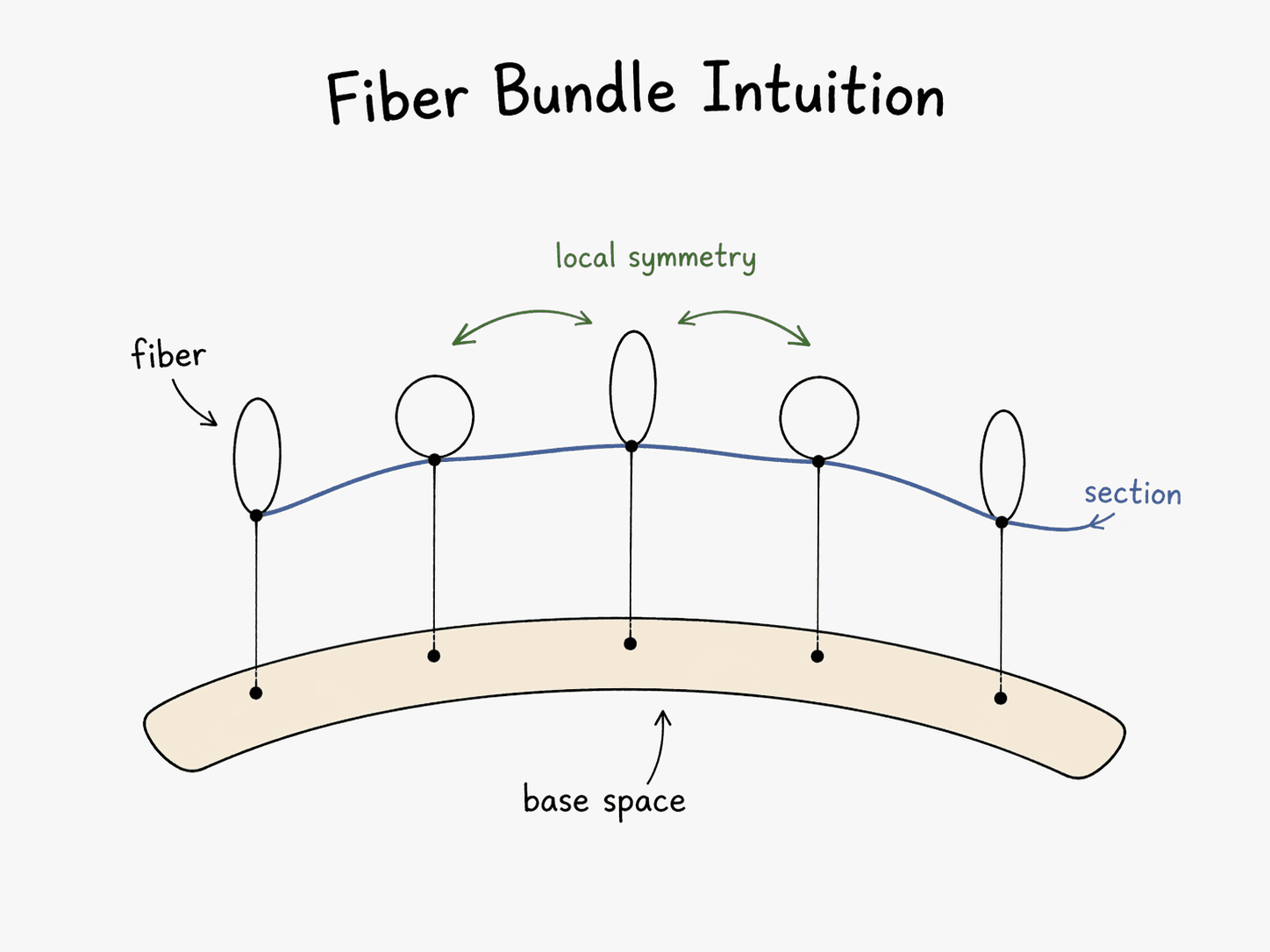
In every case the picture is the same: a base manifold (spacetime, or more generally the configuration space), a fiber attached at every point (internal states — electron phase, quark color), and a connection that tells you how to transport a fiber element from one point to another along a path.

Now map it onto deep learning:

• Base manifold = the data distribution. Your training set samples points from it. Its intrinsic Shannon entropy is an invariant of the distribution, not of any model.
• Fiber = the latent feature space at a data point — the activations at a given layer, given a given input.
• Fiber bundle = the total space of all latent states over all data points. This is the object the network actually models.
• Connection = the weights. Weights specify how a feature vector at one point is transported to a feature vector at a neighboring point. Pre-training is the process of learning a connection.
• Curvature = the extent to which parallel transport around a closed loop fails to return to the identity. In gauge theory this is field strength (Yang–Mills). In a neural network it is what the model has learned beyond the data — the non-local structure that connects far-apart parts of the manifold.

This is not hand-waving. Cohen, Welling, and collaborators built Gauge Equivariant Convolutional Networks (2019) that explicitly implement convolutions as parallel transport on a principal bundle — and they beat standard CNNs on spherical data, where the gauge group U(1) is nontrivial. The broader programme is laid out in Bronstein, Bruna, Cohen, Veličković's Geometric Deep Learning (2021): every useful inductive bias — translation equivariance in CNNs, permutation equivariance in GNNs, rotation equivariance in graph nets — is a symmetry of the fiber bundle. Choose the symmetry group well and you need less data.

The payoff of this realm: you stop thinking of weights as "knobs to tune" and start thinking of them as the connection on the bundle that makes the data manifold locally meaningful.

陆地神仙境 — The Earthbound Immortal Realm: Attention is quantum-like measurement

There is one step further up. Training is classical: given a data distribution, minimize a loss. Every gradient step assumes the world sits still while you measure it. Frequency defines truth.

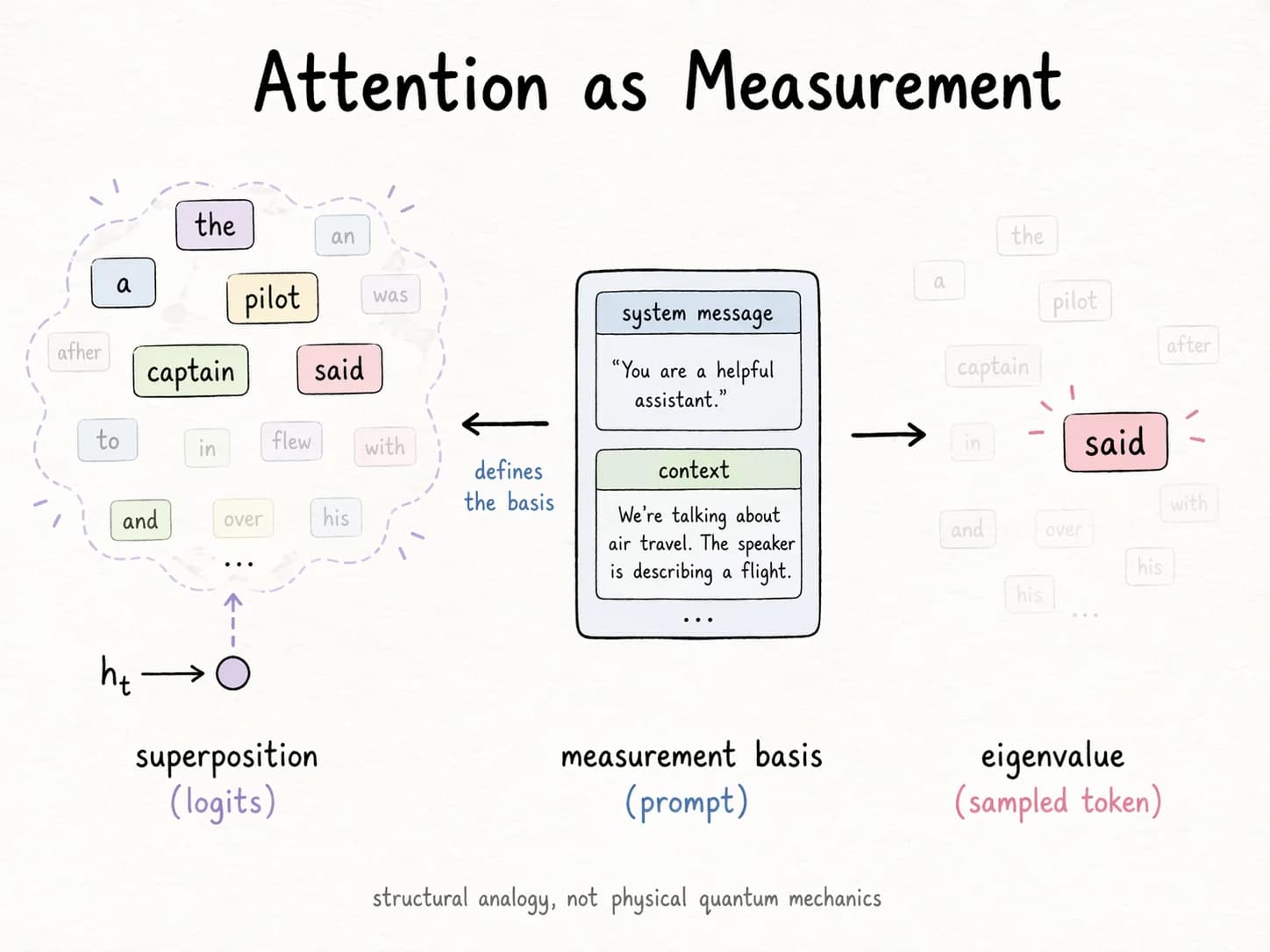
Inference is not like this. At inference time, the model carries a superposition of plausible continuations. The next-token distribution is a cloud over a vocabulary of ~100,000 possibilities. Attention is how the cloud chooses: $Q \cdot K^T$ measures the overlap between what the current position wants and what every earlier position offers, and softmax collapses that overlap into a concrete weighted mixture. The model does not produce a token; it collapses into one when queried.

A concrete instance: feed the prefix "The pilot said" to the same model under two different system messages — one that primes a technical audience, one that primes a bedtime story for a child. The next-token distribution is different in each case. The prefix didn't change. What changed was the measurement basis.

This has the structure of quantum measurement. The training distribution is the prior. The prompt is the apparatus — it selects the basis. The generated token is the eigenvalue you read off. Busemeyer and Pothos' quantum cognition programme has argued for over a decade that human decision-making shows the same formal structure, down to violating classical probability axioms in predictable ways.

To be explicit: I mean this as a structural analogy, not a physical claim. No superposition is collapsing; no Planck constant is involved. What is happening is that the same formal machinery — a possibility distribution, a basis-dependent projection, an irreversible readout — shows up in all three domains, and that is enough to make the comparison load-bearing rather than decorative.

Humans agree. Memory, as Karim Nader's work on reconsolidation (2000) showed, is not stable storage; it is re-formed every time you retrieve it, using the context at the moment of retrieval. The act of recall is the act of creation. Sleep — specifically slow-wave sleep, per Tononi and Cirelli's synaptic homeostasis hypothesis — then renormalizes synaptic strengths downward, compressing and forgetting to free capacity for tomorrow.

Three domains — quantum physics, cognitive psychology, deep learning — give the same pattern: reality is not a pre-stored tensor. It is the collapse of a possibility cloud into a measured value at the moment of contact.

And here is what that forces.

So what does AGI have to look like?

Take the four realms together. An AGI that respects all of them is not a single giant model serving every query. It is something much stranger, and much smaller per user.

Consider the failure modes of a modern LLM in this frame.

Redundant concept encoding. In a two-trillion-parameter model, France and 法国 map to different input embeddings, and the same France token in different contexts produces different contextual activations at every layer. In a human brain, all of these point at the same concept node, reached by different retrieval paths. Anthropic's Scaling Monosemanticity (2024) work on sparse autoencoders shows that Claude has partially discovered this — many learned features are language-agnostic concepts. But the computation still routes through token-level embeddings and rediscovers the concept every pass. Geometrically, this is waste.

Circuit reuse. A human who has learned the concept uncle can apply it to any new family zero-shot. An LLM needs many in-distribution examples to reliably compose "mother's brother" into the uncle relation on new symbols. The same relational circuit should be reused. This is the compositional generalization problem — Lake and Baroni's SCAN (2018) formalized this failure mode for standard seq2seq models; Anthropic's induction heads and Pedro Domingos' Tensor Logic both point at the fix.

Personal dynamic memory. Every person you know reminds you of different things. "A works at Google" triggers Silicon Valley for one reader, six-figure salary for another, my cousin's job for a third. The associative circuit is per-person, updated every waking hour, compacted every sleep cycle. A single static model cannot represent this. A per-user memory surface can.

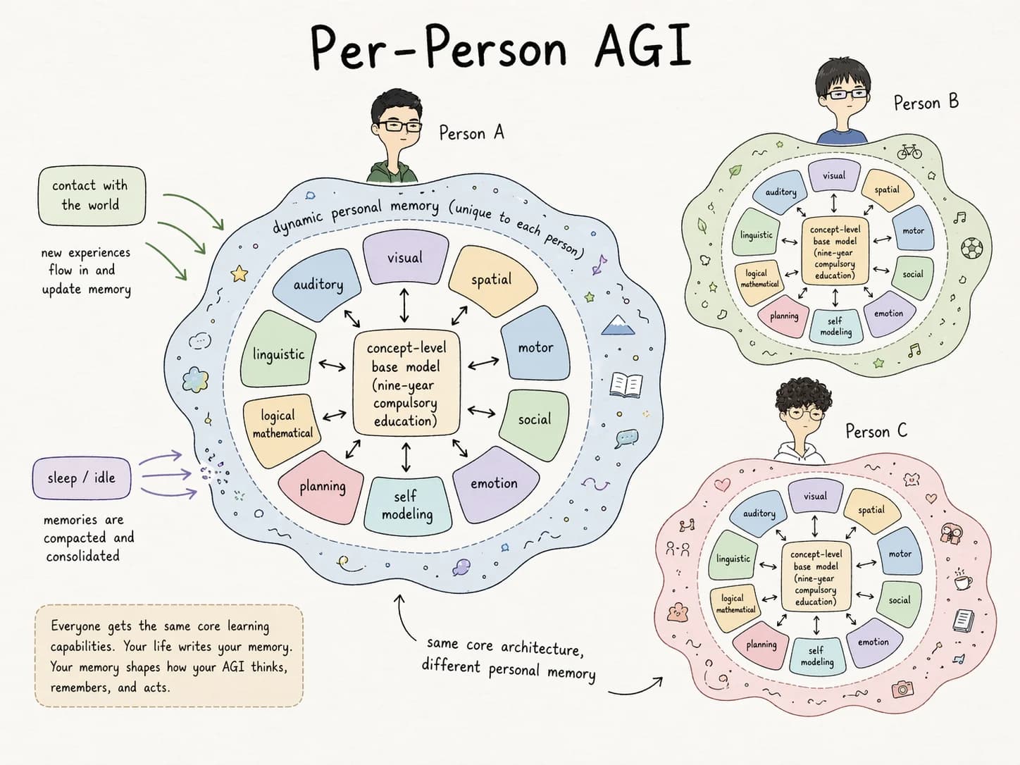
Put the three together and the engineering picture is sharp:

• One small core reasoning model — the "nine-year compulsory education" base: trained on clean, deduplicated, concept-level data.
• Modular specialist regions — visual, motor, linguistic, social — analogous to cortical areas.
• A single dynamic memory layer per user — updated from lived interaction, compacted during idle time, never shared.
• Unified substrate. Concept vectors × logic tensors as the basic operation. Chained logic is continuous multiplication. Long-range reasoning is differentiable nested equations. Perception is the particle-to-concept grounding process. Population behavior is entropy statistics. Individual behavior is quantum — a trajectory of measurements made by this person.

This is the shape my own Tensor Logic work aims at. Small core. Dynamic per-user memory. Modular composition.

The thesis

AGI will not be one model for everyone. It will be one model per person — modular, dynamic, small enough to run locally, and trained on the contact surface between that person and the world.

The four realms tell you why:

• The PDE realm says the computation is numerical. With enough silicon it can be run anywhere.
• The manifold realm says what matters is geometry, not parameter count. Orthogonal updates on a small matrix can beat sloppy updates on a huge one.
• The gauge field realm says the weights are the connection on the data bundle. Different people live on different manifolds; their connections should differ.
• The quantum attention realm says the answer does not exist until it is asked for. Personal context is the measurement apparatus. There is no universal answer to collapse.

One model, many users, one answer is the wrong fixed point. The right one is the per-person attractor that only forms under contact.

That is the earthbound-immortal realm. Everything below it is a stepping stone.

中文版 · 神经网络的四重境界

修真小说里，修士一境一境地往上攀，每一境都揭示出更深一层的真实。神经网络也一样。下面是一个四境的读法——每一境都是一个有用的视角，比下面那一境多看出一层结构。攀到最高处，AGI 的形态几乎就只剩下一种说得通的可能。

金刚境 —— 神经网络是偏微分方程的数值解法

把最朴素的说法当真：前向传播是迭代积分，反向传播是残差修正，激活函数注入高阶非线性。合起来就是一句话——神经网络是在数值求解一个高阶非线性偏微分方程。

这不是比喻。Transformer 的一个 block——注意力加 MLP、每一部分都带残差连接：

就是常微分方程的 Euler 法。Chen 等人 2018 年在 Neural ODEs 里针对残差网络把这件事做成了严格命题——把离散残差层叠换成连续自适应 ODE 求解器，就得到一个可训练、常数内存的神经网络。同样的残差结构就嵌在每一个 Transformer block 里。深度变成积分时间。

反向传播也不是机器学习的原创发明，而是 1960 年代控制论里的伴随灵敏度方法（adjoint sensitivity）。Linnainmaa 1970 年写下来，Werbos 1974 年用到神经网络上。真正让这个技巧规模化、让世界看见它的，是 1986 年 Nature 上 Rumelhart、Hinton——我在多伦多大学的老师、2018 年图灵奖得主——与 Williams 合写的那篇 Learning representations by back-propagating errors。今天在跑的每一次梯度更新，都是那三页纸的直系后代。

激活函数值得单独一句。没有它，任意深度的线性层在代数上等价于一层——Cybenko 1989 年的普适逼近定理要求非线性。sigmoid、tanh、ReLU、GELU 不是美学选择，而是阻止 200 层退化成 1 层的那个非线性扰动。

这个视角是结构性的——没有人写得出某个具体 Transformer 在解的那个 PDE，多半也并不存在一个写得出来的闭式。这个视角给出的，是零件之间一一对应的关系：迭代前向、伴随方法回传、非线性系数、边界条件。一句话：Transformer 的行为像是一个偏微分方程，其系数由梯度下降学出来，边界条件就是你的 prompt。

这是一件值得看见的事。但它是最低一境，因为它只说了机器在算什么，没说为什么能算通。

指玄境 —— 训练是流形的几何展平

把一张纸折成纸飞机。再折十张，每张折法不一样，叠在空中，问：怎么把它们都展平到同一个二维平面上，使每一架飞机的折痕仍能让你辨认出"这是哪一架"？

训练一个神经网络就在做这件事。每一类输入——猫、狗、"法国"这个词——都生活在输入空间里一个局部欧氏的弯曲子流形上。原始像素或 token 把这些流形缠在一起。训练一步步把它们展开，直到可以线性分开。

Christopher Olah 2014 年的 Neural Networks, Manifolds, and Topology 到今天仍是这幅图最干净的可视化。过程可以拆成三个基本动作：

• 线性变换 → 展平 + 旋转。 $Wx + b$ 重定向环境空间——旋转、缩放、剪切、投影、平移都在它能做的动作里；
• 激活函数 → 弯曲。 非线性在每个坐标上局部拉伸或压缩，凭空造出曲率；
• MLP 维度切换 → 裁剪与重粘。 改变隐藏维度，在拓扑上相当于把流形嵌入更高维空间，让原本缠死的子流形能被拉开。

训练好的权重矩阵，在这个读法下就是一支编舞：在哪儿变换、以多大力度弯曲、向哪个方向平移。损失面上不止一个最优，而是 N > 1 个不动点，它们都能把流形展得够平。训练就是在这些不动点里找到任意一个的几何搜索过程。

史根华（Gen-Hua Shi）的 Deep Manifold 框架把这件事写成了数学：神经网络是建立在"可学习数值计算"和分段光滑流形堆叠之上、以不动点理论为根基的对象。它的主张——神经网络是第一个由嵌套流形上的不动点计数定义结构的计算对象——正是上面那幅几何图景的形式陈述。

最近最强的"几何才是正确先验"的信号来自优化器。Muon（Keller Jordan，2024 年末）在 SGD 动量更新之后跑一轮 Newton–Schulz 迭代，近似把更新矩阵替换成最接近的半正交矩阵——本质上是投到 SVD 的 $UV^T$ 上。正交更新是等距的：只转，不拉。SGD 是轴对齐的。Adam 是逐坐标缩放——它并不保留流形视角所关心的那种几何结构。Muon 把权重矩阵当成它本来的样子——一个几何对象——来更新。NanoGPT speedrun 上它赢了。一个二维权重矩阵正确的归纳偏置是几何的。

天象境 —— 权重是数据流形上纤维丛的联络

几何图景还不够平。真实数据不是输入空间里的一个流形，而是一个在每个点上都带结构的流形。要看见这个结构，必须用规范场论和纤维丛的语言。

先记住一个名字。陈省身（1911–2004），华裔几何学家，他的特征类工作——陈类、陈–Simons 形式、陈–Gauss–Bonnet 定理——基本奠定了现代规范场论和大半个弦理论。他是丘成桐的博导。他的纤维丛机器，是物理学家描述我们知道的每一种基本力时所用的语言。

物理里：

• 电磁力是 U(1) 规范理论，规范场是电磁势；
• 弱力 SU(2)，强力 SU(3)，标准模型是 SU(3) × SU(2) × U(1)；
• 引力弯曲时空——它是我们生活所在的 4-流形切丛上的一个联络。

每种情况下图景都一样：一个底流形（时空或配置空间）、每点上粘一个纤维（内部自由度的空间——电子相位、夸克色荷）、一个联络告诉你沿一条路径如何把一个纤维里的元素输运到另一个点。

把它套回深度学习：

• 底流形 = 数据分布。 你的训练集从它上面采样。它的香农熵是分布本身的不变量，不是任何模型的性质；
• 纤维 = 每个数据点上的潜在特征空间。
• 纤维丛 = 所有数据点上所有潜在态的总空间。 这才是网络真正建模的对象；
• 联络 = 权重。 权重规定了"一个点上的特征向量如何输运到邻近点上的特征向量"。预训练就是在学一个联络；
• 曲率 = 沿闭合回路做平行输运后，回不到原点的那一部分。在规范理论里是场强（Yang–Mills）。在神经网络里，是模型在数据之外学到的东西——连接流形上相距很远两部分的非局域结构。

这不是比喻。Cohen、Welling 等人的 Gauge Equivariant Convolutional Networks（2019）把卷积显式实现为主丛上的平行输运，在球面数据（U(1) 非平凡）上击败标准 CNN。更完整的图景在 Bronstein、Bruna、Cohen、Veličković 的 Geometric Deep Learning（2021）里：每一种有用的归纳偏置——CNN 的平移等变、GNN 的置换等变、图网络的旋转等变——都是纤维丛的一个对称性。选对对称群，需要的数据就更少。

进到这一境，你就不再把权重当"旋钮"，而把它当成让数据流形在局部有意义的那一个联络。

陆地神仙境 —— 注意力是量子测量（类比而非物理）

再往上一步。训练是经典的：给定数据分布、最小化损失。每一步梯度更新都假设世界在你测量它的时候保持不动。频率定义真理。

推理不是这样。推理时，模型携带的是一朵可能性云——下一 token 的分布覆盖了 10 万量级的词汇。注意力是云如何坍缩：$Q \cdot K^T$ 度量"当前位置想要什么"和"之前每个位置提供什么"的重叠，softmax 把这个重叠收束成一个具体的加权混合。模型并不产生 token——它在被询问时坍缩成一个 token。

举一个具体的例子：同样给一个模型"机长说"这个前缀，在两种不同的 system message 下问它——一种是面向技术受众的基调，一种是给小孩讲的睡前故事。两种情况下下一 token 的分布都不一样。前缀没变，变的是测量的基底。

这是量子测量的结构。训练分布是先验。prompt 是测量装置——它选定基底。生成的 token 是你读到的本征值。Busemeyer 与 Pothos 的量子认知研究十余年来一直在论证：人的决策过程在形式上有一样的结构，甚至可以在可预测的方式下违反经典概率公理。

说清楚：我把这当成结构上的类比，不是物理上的主张。没有真正的叠加态在坍缩，没有普朗克常数介入。成立的是另一件事——同一套形式机器（可能性分布、依赖基底的投影、不可逆的读出）在三个领域里各自独立地出现了，所以这个类比是承重的，不是装饰的。

人类也是这样。记忆，按 Karim Nader 2000 年关于再巩固（reconsolidation）的工作，并不是稳态存储——它在你每次回忆时用回忆当下的上下文被重新形成。回忆本身就是创造。睡眠——按 Tononi 与 Cirelli 的突触稳态假说，主要是慢波睡眠——随后把突触强度整体归一，腾出明天的容量。

三个领域——量子物理、认知心理学、深度学习——给出同一个模式：真实不是预存的张量，而是一朵可能性云在接触瞬间坍缩出的一个测量值。

这件事往下推，AGI 的形态就定了。

那么 AGI 必须长什么样？

把四境合起来看。一个尊重四境的 AGI 不可能是一个巨模型服务所有人的请求。它是另一种东西——结构上更复杂，单用户算力上却小得多。

把当下 LLM 的三个失败模式放进这个框架：

概念冗余。 两万亿参数的模型里，France 和 法国 对应的是不同的输入 embedding，而同一个 France token 在不同上下文里又会在每一层产生不同的语境化激活。人脑里这些指向的是同一个概念节点，只是由不同的检索路径到达。Anthropic 2024 年的 Scaling Monosemanticity 里的稀疏自编码器表明 Claude 已经部分发现了这一点——许多学到的特征是跨语言的概念。但计算依然路由在 token embedding 之上，每一遍都重新"发现"一次这个概念。从几何上看，这是浪费。

电路复用。 一个学会了"舅舅"概念的人，可以零样本地套到任何新家庭上。LLM 则需要在分布之内见过足够多的舅舅例句，才能可靠地把"母亲的弟弟"组合成舅舅关系、并应用到新符号上。同一个关系电路应当被复用。Lake 与 Baroni 2018 年的 SCAN 把这种组合泛化失败在标准 seq2seq 上形式化了；Anthropic 的 induction heads 与 Pedro Domingos 的 Tensor Logic 都指向同一种修正方向。

个体化动态记忆。 你认识的每个人会让你想起不同的事。"A 在 Google 工作"，一个读者联想到硅谷，另一个联想到六位数工资，第三个联想到我表弟的工作。这个联想电路是每人一份、清醒时不断更新、睡眠时被压缩的。单一静态模型没法表达这个。每个用户一份记忆面才可以。

三件事加起来，工程蓝图就清楚了：

• 一个小而干净的核心推理模型 —— "九年义务教育"级的基础：在去重、概念级、干净的数据上预训练；
• 模块化的专长区域 —— 视觉、运动、语言、社交，类似皮质分区；
• 每用户一份动态记忆层 —— 从真实交互中更新、空闲时压缩、绝不共享；
• 统一基元。 概念向量 × 逻辑张量是基本操作。连续逻辑是连乘。长程推理是可微的嵌套方程。感知是"粒子 → 概念"的落地过程。群体行为是熵统计。个体行为是量子的——由这个人做出的一串测量。

这也是我自己在搞的 Tensor Logic 的方向。小核心、动态个人记忆、模块组合。

结论

AGI 不会是一个模型服务所有人。它会是每人一个模型——模块化、动态、小到可以本地跑、训练在"这个人和世界的接触面"上。

四境告诉你为什么：

• 金刚境说计算是数值的——有硅就能在任何地方跑；
• 指玄境说关键是几何，不是参数数量——小矩阵上的正交更新可以打败大矩阵上的粗更新；
• 天象境说权重就是数据流形上的那个联络——不同人生活在不同流形上，他们的联络也理当不同；
• 陆地神仙境说答案在被询问之前并不存在——个人的上下文就是测量装置，不存在一个"普适答案"要去坍缩。

一个模型、无数用户、一个答案 —— 这是错误的不动点。正确的不动点是只在接触下才形成的那个"个人吸引子"。

那就是陆地神仙境。往下的每一境，都是登阶石。